Value Creation is essential in Private Equity.
In the context of Private Equity, Value Creation is defined as the set of post-investment activities aimed at generating a positive return for the PE manager, or equivalently increasing the value of the private company that was acquired.
In simpler terms, the PE Manager implements Value Creation activities in order to sell a company at a higher price than what he paid at time of acquisition.
This article aims first at explaining how Value Creation can be measured, and decomposed into its four main components. Thereafter, we will try to interpret the results and extract information about the Private Equity manager skill set, and its potential improvement areas.
Measuring Value Creation
The outcome of Value Creation (in essence, the return for the Private Equity manager) can be quantified by employing two similar indicators:
- The Internal Rate of Return – IRR
- The Cash on Cash multiple – CoC
The IRR can be thought as a time-weighted percentage return between the moment of purchase and the moment of sale of a private company. The CoC – instead – ignores the time dimension and it is simply the ratio between the sales proceeds and the money invested at entry.
Both indicators can be measured at deal level (i.e. a single investment into one company) or at portfolio level (i.e. a number of investments into several companies).
Value Creation Components
While the IRR and the CoC indicators offer a quick numerical approximation about about the success of a private equity deal or a portfolio of private equity deals, they do not provide any insight on the actual sources of value creation. To get additional insight, we have to decompose them.
Let us start by identifying the four main components of Value Creation, into which we want to break down the chosen numerical indicator. They are:
- OPERATIONAL IMPROVEMENT – Was the PE manager particularly good at managing the Company’s operations (measured by the Company’s Sales and its EBITDA margin)?
- USE OF FINANCIAL LEVERAGE – Did the PE manager generate equity returns through the use of debt (measured by the Equity to Assets ratio)?
- MARKET TIMING – Was the PE manager lucky (or skilled) in identifying market timing, buying cheap and selling expensive (measured by the EV to EBITDA multiple)?
- FOREIGN CURRENCY EFFECT – Was the PE manager favoured or penalised by the relative appreciation of the Company’s operational currency (measured by the FX rate differential vs. hard currency)?
The first component, OPERATIONAL IMPROVEMENT, can be in turn broken down into two metrics:
- SALES – improvement of top-line performance, generally achieved by increasing volumes and prices
- EBITDA MARGIN – improvement of bottom-line profitability, generally achieved by cost savings and operational efficiencies
To decompose the IRR into the four factors above, we use a mathematical technique similar to the DuPont Analysis, which we outline below.
IRR Decomposition
As a reminder (disregarding dividends) we said we can think about the IRR as a time-weighted percentage difference between the value of an equity stake at entry and its value at exit.
Statically, the equity value can be expressed as follows for a corporate:
E_{\$} = (Sales_{ccy} \cdot EBITDAmargin) \cdot \frac{EV_{ccy}}{EBITDA_{ccy}} \cdot \frac{E_{ccy}}{EV_{ccy}} \cdot FX_{\$/ccy}The first term of the equation represents a Company’s operating performance (Sales multiplied by the EBITDA margin returns the Company’s EBITDA = Earnings Before Interests, Taxes, Depreciation and Amortisation). The change through time of Sales and EBITDA margin corresponds to the OPERATIONAL IMPROVEMENT Value Creation component.
The second term of the equation represents the market valuation of the company (in its ratio Enterprise Value to EBITDA). Its change through time corresponds to the MARKET TIMING Value Creation component.
The third term of the equation represents a measure of leverage (the Equity to Enterprise Value ratio). Its change through time corresponds to the USE OF LEVERAGE Value Creation component.
The fourth term of the equation represents the translation between local currency and hard currency. Its change through time corresponds to the FOREIGN EXCHANGE Value component.
For a Financial Institution (bank or insurance company), the formula varies slightly: EBITDA is replaced by Total Assets, the EV / EBITDA ratio is replaced by E/NAV (or Price to Book value), the relative leverage is changed into NAV / Assets:
E_{\$} = Assets_{ccy} \cdot \frac{NAV_{ccy}}{Assets_{ccy}} \cdot \frac{E_{ccy}}{NAV_{ccy}} \cdot FX_{\$/ccy}In order to determine the time-weighted percentage difference of the entry and exit equity value (which we called IRR) and analyse dynamically the relative contribution of the 4 components, we compute compounded annual growth rates (CAGRs) on both sides of the above formula. We get (shown for corporates only):
1 + CAGR(E) = [1+CAGR(Sales)] \cdot [1+CAGR(EBITDAmargin)] \cdot
[1+CAGR(\frac{EV}{EBITDA})] \cdot [1+CAGR(\frac{E}{EV})] \cdot [1+CAGR(FX)]
Note: When EBITDA margin is negative, the equation loses significance. In those cases, we use only Sales as a reference for the operational improvement: E=Sales \cdot \frac{EV}{Sales} \cdot \frac{E}{EV} \cdot FX
To obtain an “addition format” in the equation, we first take logarithms and then divide both sides by the natural logarithm of 1+IRR(E). In formula:
100\% = \frac{ln[1+CAGR(Sales)]}{ln[1+IRR(E)]} + \frac{ln[1+CAGR(EBITDAmargin)]}{ln[1+IRR(E)]}+
\frac{ln[1+CAGR(\frac{EV}{EBITDA})]}{ln[1+IRR(E)]} + \frac{ln[1+CAGR(\frac{E}{EV})]}{ln[1+IRR(E)]} + \frac{ln[1+CAGR(FX)]}{ln[1+IRR(E)]}
Because these terms add up to 100%, they can now be interpreted as the relative contribution of the FOUR components to the totality of our Equity IRR for each investee company we have in our portfolio.
Equivalently:
100\% = (Sales\cdot margin)growth + Multiple expansion + Leverage + FX .Interpreting the results
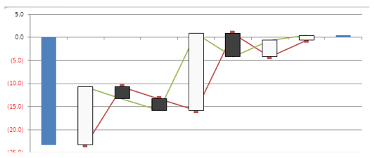
The IRR decomposition process can be aptly visualised in a waterfall chart, similar to the one below:
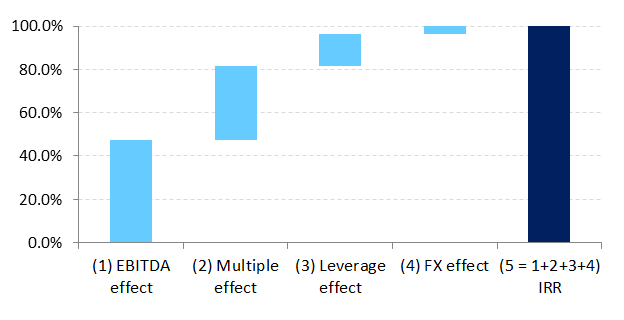
Whether we are analysis a single deal, or a portfolio, we would ideally like each of the components to be positive. If that is the case, we can say that the PE manager is able to create value throughout the full value creation range: he improved the operations of a company, was able to use leverage effectively, was able to buy at a multiple cheaper than what he sold and was favoured by the movements of the FX rate vs. USD.
The worst case scenario is instead when all value creation components are negative: in that case, the PE manager has destroyed value throughout.
In reality, however, it is common to see that some components will be negative even when the overall deal IRR is positive. In particular, Sales and EBITDA margin improvement tend to be negatively correlated with the market timing: as the company matures, the market is willing to pay a lower multiple (discounting future lower growth).
Also, to assess the PE Manager performance, it will be important to assess to what extent the above-mentioned parameters are under his/her full control.
The below table will provide some reference:
| Value Creation Component | Extent of Control |
|---|---|
| Operational Improvement | FULL |
| Market Timing | MEDIUM |
| Leverage | FULL |
| FX | LOW |
With the guidance above, we come to an important conclusion: the success of the Private Equity manager can be primarily assessed on the way he/she creates value via enhancing the company’s operations and using financial leverage effectively. The market timing and FX component – however important – are under less control of the manager and therefore will only be second-degree parameters when assessing his/her performance.
We invite you to run the analysis on your PE managers’ portfolios, or even on a whole set of industry deals over a given time horizon to attribute the private equity returns to a given Value Creation component.
Methodological Remarks
This methodology is intuitive and simple. This is its key advantage. However, as usual for a data aggregation, simplicity comes at the expense of precision.
The main disadvantages of the value creation decomposition methodology we designed are:
- Disregards the impact of dividends and interim capital distributions. However, the bulk of private equity returns [and losses] is traditionally obtained by the capital gain between entry and exit. In most of the PE deals, interim distributions play only a minor part in the determination of the actual Internal Rate of Return
- At a portfolio level, the aggregation of deal-level results needs to be performed using a relatively large sample (at least 30 observations). Not many PE manager will have that many companies in their portfolio.
- The IRR goes to minus infinity if all money is lost (e.g. the Company may go bankrupt and there is no residual equity value left). While this is an issue, still the value creation decomposition can identify the causes of failure even when the IRR is deeply negative.
- Looks at returns from a company equity-value perspective and not individual shareholders’ perspective. In the instances that an individual shareholder makes more than one capital contribution at different valuations, the value creation formula will have to be adjusted to take this into account in a non-trivial manner
References:
- Acharaya, Viral V., Oliver Gottschalg, Moritz Hahn, and Conor Kehoe, 2011. “Corporate Governance and Value Creation: Evidence from Private Equity”. Available at SSRN: http://ssrn.com/abstract=1324016.
- Achleitner, Ann-Kristin, Reiner Braun, Nico Engel, Christian Figge, and Florian Tappeiner. 2010. “Value Creation Drivers in Private Equity Buyouts: Empirical Evidence from Europe”. Journal of Private Equity 13, 17–27.
- Axelson, Ulf, Tim Jenkinson, Per Strömberg, and Michael S. Weisbach, 2010. “Borrow Cheap, Buy High? The Determinants of Leverage and Pricing in Buyouts”. Available at SSRN: http://ssrn.com/abstract=1596019.
- Diller, Christian, and Christoph Kaserer. 2009. “What Drives Private Equity Returns? – Fund Inflows, Skilled GPs, and/or Risk?.” European Financial Management 15, 643–675.
- Gompers, Paul A., and Josh Lerner, 2000. “Money Chasing Deals? The Impact of Fund Inflows on Private Equity Valuations.” Journal of Financial Economics 55, 281- 325.
- Guo, Shourun, Edith S. Hotchkiss, and Weihong Song, 2011. “Do Buyouts (Still) Create Value?”. Journal of Finance 66, 479-517.
- Jenkison, Tim, and Rüdiger Stucke, 2010. “Who Benefits from the Leverage in LBOs?”. Available at SSRN: http://ssrn.com/abstract=1777266.
- Kaplan, Steven N., and Antoinette Schoar. 2005. “Private Equity Performance: Returns, Persistence, and Capital Flows.” Journal of Finance 60, 1791–1823.
- Kaplan, Steven N., and Per Strömberg. 2009. “Leveraged Buyouts and Private Equity.” Journal of Economic Perspectives 23, 121–146.
- Kaserer, Christoph, 2010. “Return Attribution in Mid-Market Buy-Out Transactions – New Evidence from Europe” CEFS Research Report Series. Available at http://ssrn.com/abstract=1946110
- Nikoskelainen, Erkki, and Mike Wright. 2007. “The impact of corporate governance mechanisms on value increase in leveraged buyouts.” Journal of Corporate Finance 13, 511–537.
- Phalippou, Ludovic, and Oliver Gottschalg. 2009. “The Performance of Private Equity Funds.” Review of Financial Studies 22, 1747–1776.